
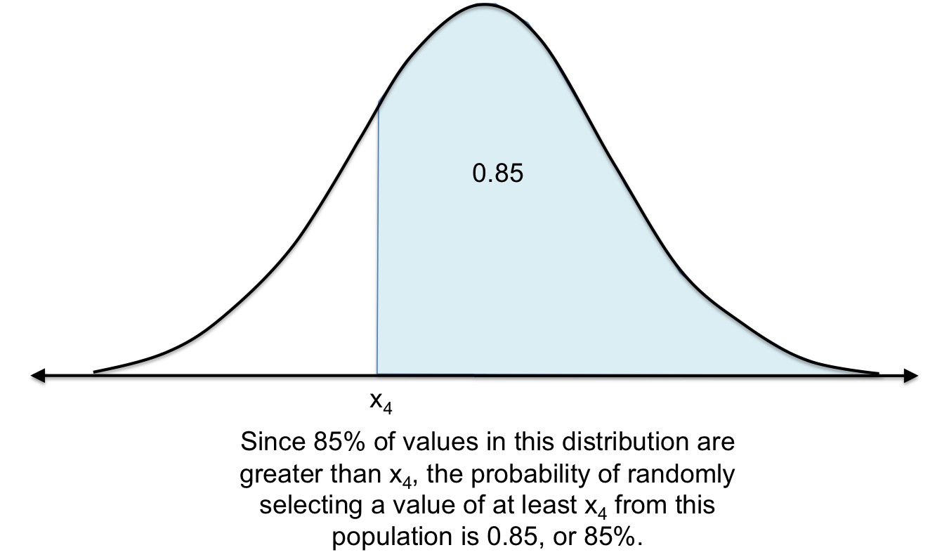
Now that you know the standard way we describe the location of values on a normal distribution, we can find the proportion less than or greater than a certain value.
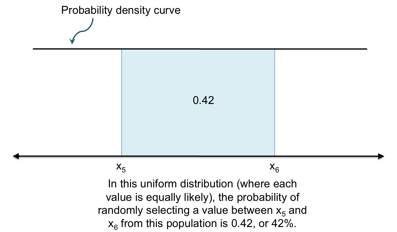
Since the total area under the curve is 1 (meaning, 100% of the population is part of this distribution), the area between any two points is equal to the proportion of values in-between those two points, which is essentially the probability of randomly selecting a value from that population between those two points.
For this reason, smooth distributions modeled by these curves are called probability distributions because the area beneath represents the approximate probabilities of selecting a particular value from that population. The actual curve is called the probability density curve or probability density function (PDF).
Another way to look at probabilities is with a cumulative density function (CDF), which shows the relationship between each value (x-axis) and the proportion of values less than that value (y-axis).
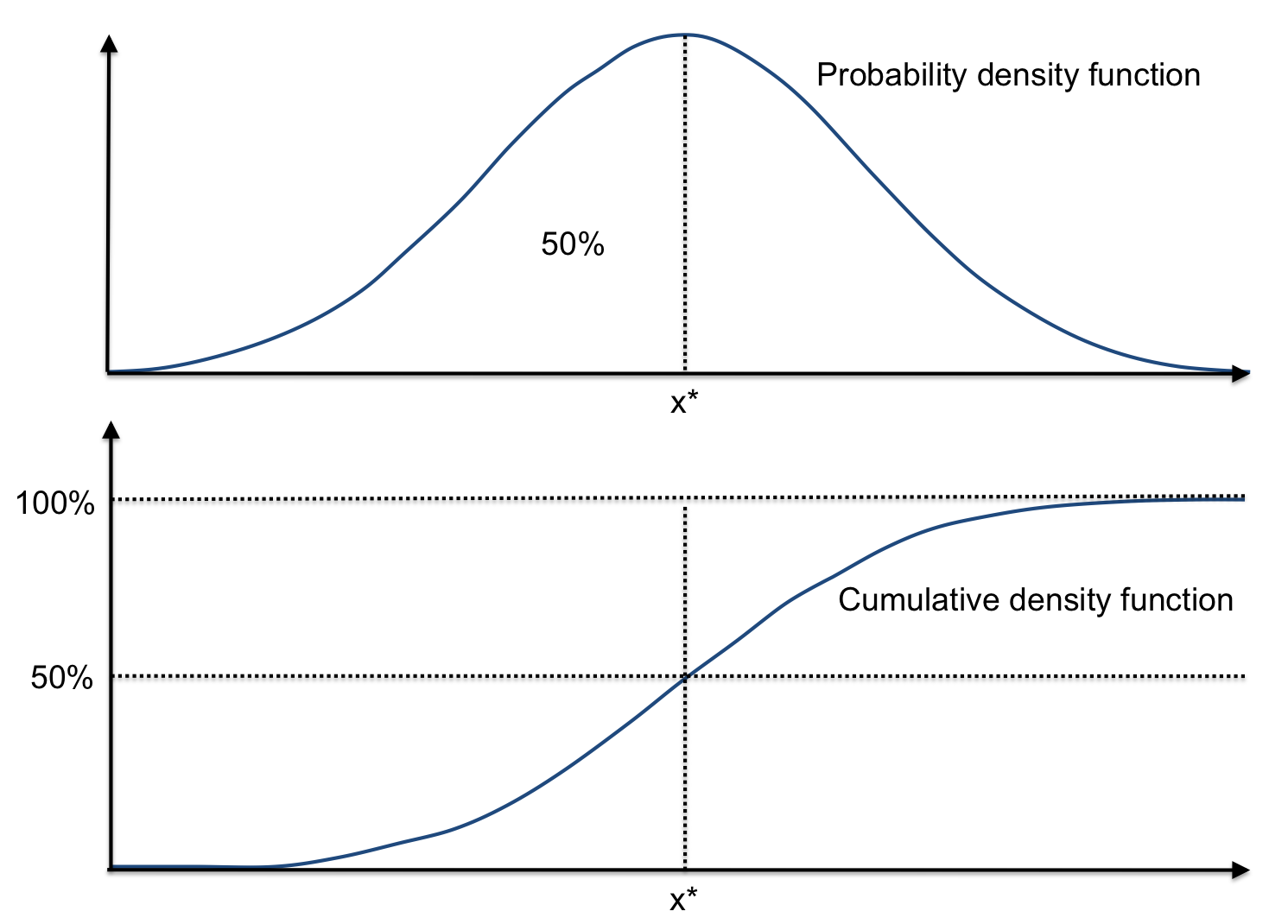
In the figure above, the bottom graph is the CDF for the normal PDF above. You see in the PDF that 50% of values are less than x*, and you can see this also with the CDF: the y-value for x* is 50%.
This is a preview of Lesson 6. To access the full book, please purchase a hard copy or a digital version. If you opt for the digital version, you will receive a link via email within 1 business day.
Continue to Lesson 7, or select a lesson below.
Lesson 1: Introduction to Statistical Research Methods
Lesson 2: Visualizing Data
Lesson 3: Central Tendency
Lesson 4: Variability
Lesson 5: Standardizing
Lesson 6: Normal Distribution
Lesson 7: Sampling Distributions
Lesson 8: Estimation
Lesson 9: Hypothesis Testing
Lesson 10: t-Tests for Dependent Samples
Lesson 11: t-Tests for Independent Samples
Lesson 12: Intro to One-Way ANOVA
Lesson 13: One-Way ANOVA: Test significance of differences
Lesson 14: Correlation
Lesson 15: Linear Regression
Lesson 16: Chi-Squared Tests
Afterward
Index