
Let’s say you have these two salary distributions. They have the same mean, median, and mode.
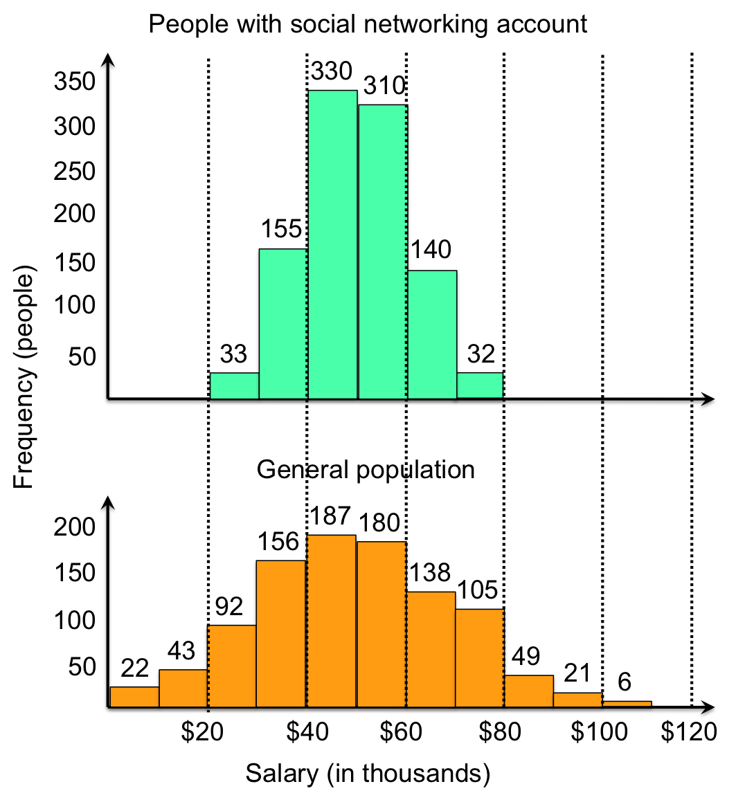
The main difference between them is the spread. One way we can see this is by looking at the range of each dataset.
The range in the top distribution is $78,600 – $21,180 = $57,420
The range in the bottom distribution is $116,020 – $7350 = $108,670
You can see from the range that the salaries of the general population are much more dispersed whereas salaries of those with social networking accounts are more concentrated.
While range is one method to describe the spread of data, it has limitations. Namely, if the data includes more people within that range, the range will not change. Take these four distributions, for example.
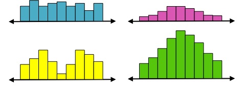
They all have the exact same range, and similar means, medians, and modes, but they all have very different shapes. The top left is relatively uniform; the top right is normal; the bottom left is bimodal; and the bottom right is also normal, but with more data points. Therefore, you see that the range itself does not adequately describe the spread of data.
This is a preview of Lesson 4. To access the full book, please purchase a hard copy or a digital version. If you opt for the digital version, you will receive a link via email within 1 business day.
Continue to Lesson 5, or select a lesson below.
Lesson 1: Introduction to Statistical Research Methods
Lesson 2: Visualizing Data
Lesson 3: Central Tendency
Lesson 4: Variability
Lesson 5: Standardizing
Lesson 6: Normal Distribution
Lesson 7: Sampling Distributions
Lesson 8: Estimation
Lesson 9: Hypothesis Testing
Lesson 10: t-Tests for Dependent Samples
Lesson 11: t-Tests for Independent Samples
Lesson 12: Intro to One-Way ANOVA
Lesson 13: One-Way ANOVA: Test significance of differences
Lesson 14: Correlation
Lesson 15: Linear Regression
Lesson 16: Chi-Squared Tests
Afterward
Index