
When there is an identifiable trend in the data (i.e., at least a moderately strong correlation between x and y), we often want to model this relationship so that we can interpolate (estimate the value of y for any given value of x within the range of data we have) and extrapolate (predict the value of y for any given value of x beyond our range of data).
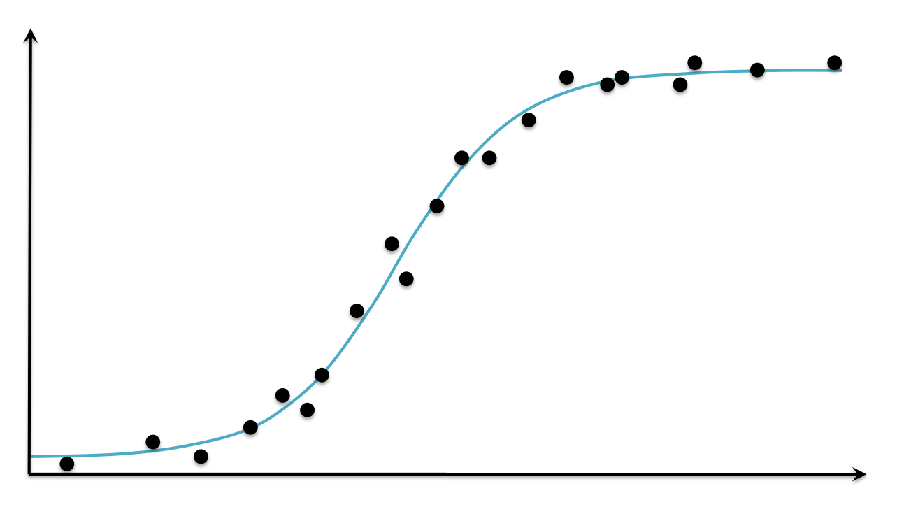
To model relationships, we can use a line or curve. The type of curve that best fits the data below is logistic.
There are many possibilities for which functions you could use to model the data, but the simplest is with a line. Therefore, this is called linear regression.

As you saw in Lesson 14, each x-value is xi and each y-value is yi. The line used to model the trend between the xi’s and yi’s is called the regression line or line of best fit.
This is a preview of Lesson 15. To access the full book, please purchase a hard copy or a digital version. If you opt for the digital version, you will receive a link via email within 1 business day.
Continue to Lesson 16, or select a lesson below.
Lesson 1: Introduction to Statistical Research Methods
Lesson 2: Visualizing Data
Lesson 3: Central Tendency
Lesson 4: Variability
Lesson 5: Standardizing
Lesson 6: Normal Distribution
Lesson 7: Sampling Distributions
Lesson 8: Estimation
Lesson 9: Hypothesis Testing
Lesson 10: t-Tests for Dependent Samples
Lesson 11: t-Tests for Independent Samples
Lesson 12: Intro to One-Way ANOVA
Lesson 13: One-Way ANOVA: Test significance of differences
Lesson 14: Correlation
Lesson 15: Linear Regression
Lesson 16: Chi-Squared Tests
Afterward
Index